MS Excel Drop-Down Lists
HOME
If you have to type the same data into cells all the time, then adding a drop down list to your spreadsheet could be the answer. In Excel, this comes under the heading of Data Validation.
In the example below, we have class of students on a drop
down list. We only have to click a cell
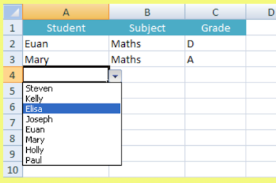
in the A column to see this same list of students. You will see how to do that now. Here is a picture of your finished spreadsheet.
In the image above, we can simply select a student from the
drop down list – no more typing. We can
also do the same for the Subject and Grade.
So, create the following headings in a new spreadsheet:
Cell A1: Student
Cell B1: Subject
Cell C1: Grade
Cell E1: Comments
We now need some data to go in our lists. So, type the same data as in the image
below. It does not need to go in the
same columns as ours. But do not type in
Columns A, B, C or E:
The data in Columns F, G, and H above will be going in to
our list.
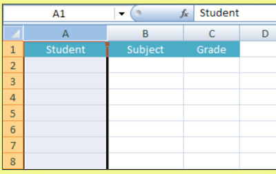
Now click on Column A to highlight that entire column:
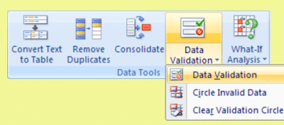
With Column A highlighted, click on Data from the Excel Ribbon at the top. From the Data tab, locate the Data Tools panel. On the Data Tools panel, click on the Data Validation item. Select Data Validation from the menu:
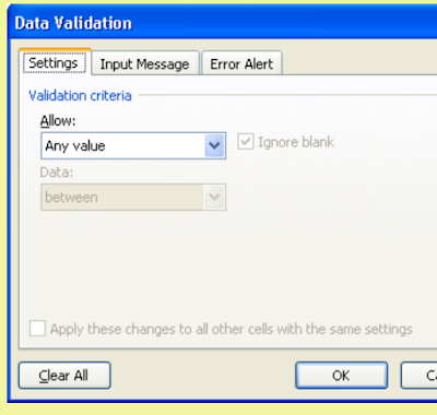
When you click Data Validation, you will see the following
dialogue box appear:
To create a drop down list, click the down arrow just to the
right of “Allow: Any value” on the Settings tab:
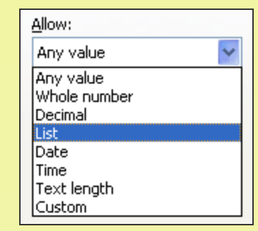
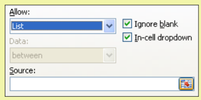
Select the List from the drop down menu, and you will see a
new area appear:
Source means,
which data you want to go in your list. You
can either just type in your cell references here or let Excel do it for you.
To let Excel handle the job, click the icon to the right of the Source text box:
When you click this icon, the Data validation dialogue box
will shrink:
Now select the cells on your spreadsheet that you want in
your list. For us, this is the Students:
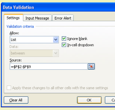
Once you have selected your data, click the same icon on the
Data Validation dialogue box. You will
then be returned to the full size one, with your cell references filled in for
you:
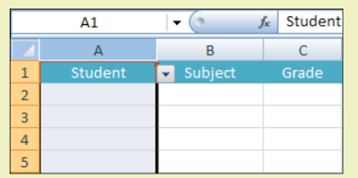
Click OK and you will see the A column with a drop down list
in cell A1:
However, you do not want to drop down list for your A1
column heading. To get rid of it, click
inside of cell A1. Click the Data
Validation item on the Data Tools
panel again to bring the dialogue box.
From the Allow list, select Any Value:
Click OK on the Data Validation dialogue box, and your drop
down list in cell A1 will be gone.
The rest of the column will still have drop down lists,
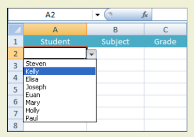
though. Try it out. Click inside cell A2 and you will see a
down-pointing arrow:
Click the arrow to see your list:
Select an item on your list to enter the name in the cell. Click any other cell in the A column and you
will see the same list.
Adding a drop down list to your cell can save you a lot of
time and it means that typing errors would not creep in to your work.
Exercise
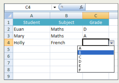
Add drop down list to the B and C columns. The B column should contain lists of
Subjects, and the C column a list of Grades.
Make sure that the cells B1 and C1 do not contiain drop down lists. Whe you are finished, the Subject column
should like this:
And the grade column should look like this:







Comments
Post a Comment